In this blog post, quadric explores the acceleration of the Non-Maximal Suppression (NMS) algorithm used by object detection neural networks such as Tiny Yolo V3. We dive into the challenges of accelerating NMS, and why quadric's approach results in best-in-class performance.
When pushed to the limit of a network, the need for accelerated processing in resource-constrained settings becomes a complex problem to solve. That is where the quadric architecture comes into play. Our architecture's combination of 4 TeraOPS (TOPS) per second and 4 million-Million Instructions Per Second (MIPS) is well-suited for accelerating an entire application pipeline at the edge. MIPS is a standard measure of a CPU's speed, while TOPS is a common measure of the capability of a Neural Network accelerator. Striking a balance between these two is critical for total algorithm performance. To demonstrate this, let's take a look at a basic example: YOLO.
You might think that since YOLO is a neural network, it can be accelerated with an NPU and the TOPS it provides in its entirety. However, this isn't the case. And the reason is not apparent. To enable a neural-network-based object detection algorithm to have clean detection, we need the help of a classical algorithm: Non-Maximal Suppression, or NMS for short.
Non-maximal suppression is a critical step in detecting objects in an image. NMS is a classical algorithm that analyzes detection candidates and keeps only the best ones. However, it is computationally expensive, making it difficult to accelerate with traditional hardware architectures. The quadric architecture addresses problems like this, and it delivers the performance necessary for resource-constrained edge performance. Our approach makes it well-suited for accelerating the entire application pipeline, including but not limited to non-maximal suppression.
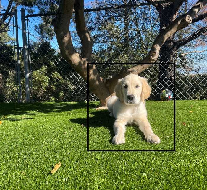
YOLO is a detection algorithm that can know if things are in an image and where. It does this by looking at the picture and deciding what it might see, for example, a person, a car, or a cat. To illustrate how detection algorithms work, let’s enlist the help of my puppy, Maverick.
A classifier algorithm may identify a dog in the photo, but it does not always indicate where in the image the pup is.

On the other hand, a localization algorithm would only tell you that something is in a position in the photograph.
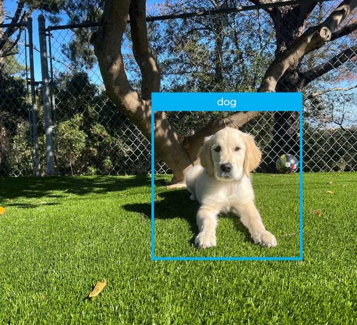
A detection algorithm will tell you a dog is in a specific image region. YOLO is one such detection algorithm.
YOLO produces a set of candidate bounding boxes around objects in an image – the boxes in which it has sufficiently high confidence that they represent the most probable dimensions and location of a recognized entity.
YOLO is more discerning than other image classification methods. It produces far fewer bounding boxes for a given object detected, and it’s faster. Let's look at YOLO in more detail. To perform the complete algorithm, technically, there are two steps:
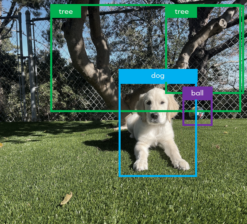
Let's start at the end: here is a nice clean image of a final detection that one would expect to see after YOLO completes a detection on an image. Dog, ball, tree. Super easy! Let’s see what it takes.
The TOPs-accelerate able NN backbone produces a set of best-guesses in the form of multiple bounding boxes, each offset around a given object, each with varying dimensions inferred by the math. Here again is Maverick framed by several bounding boxes that represent YOLOs best guesses about the sizes and probable positions of the dog in the image:
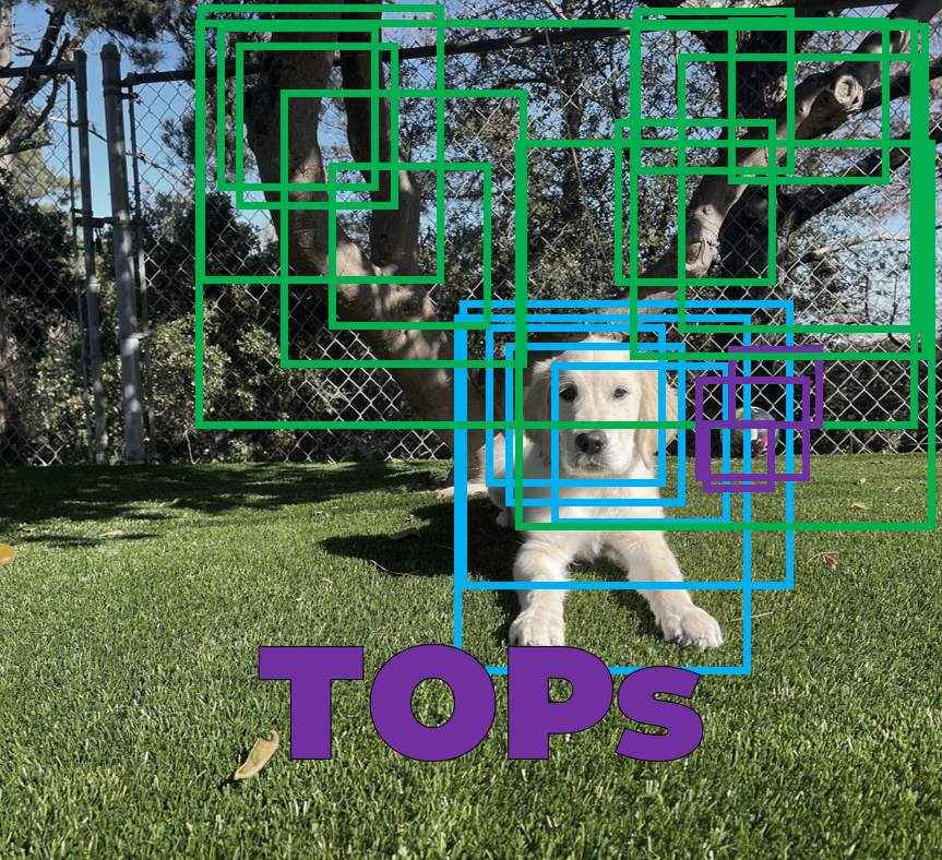
But this is as far as a TOPs-only approach using neural networks can take us.
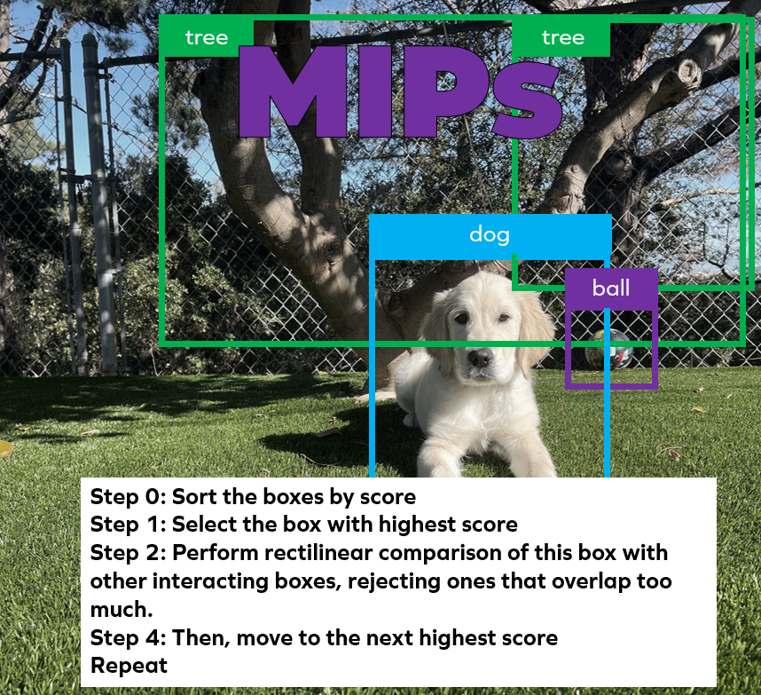
To pick the “best” box and complete the detection pipeline, we need suppression to sort boxes by their score and toss out overlapping and otherwise low-scoring boxes. The most widely used algorithm is NMS. YOLO includes NMS as a final step, as do most other detection algorithms.
So we know we need NMS. But how does it work?
NMS is a less celebrated component of the recognition pipeline. Maybe because it’s a simple, classic algorithm – or because it’s not even AI. Or perhaps it is because it is the elephant in the room: NMS is a classical algorithm that is hard to accelerate.
But that’s what makes its implementation so challenging. It’s “normal” code, built with compares, branches, loops with dynamic termination conditions, 2d geometry, and scalar math. It doesn’t run natively on an NPU and is difficult to accelerate on a GPU. NMS acceleration on a TOPs-accelerating NPU is impossible, and NMS’s acceleration on the GPU is an active research topic. NMS goes something like this:
NMS may be straightforward code-wise, but it’s a critical path component that runs in every major iteration of the detection pipeline.
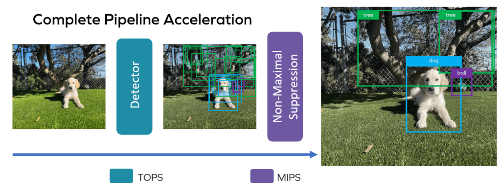
Consider the NMS implementations in TensorFlow. It provides both CPU and GPU versions, which is nice, but the GPU and CPU implementations run at about the same speed under normal conditions. State-of-the-art NMS computation execution latencies are on the order of 5-10 ms. These execution latencies are on the order of what most people would consider the more computationally intensive portion: the neural backbone. Most implementations: execute the neural backbone on an NPU or GPU, transfer the data over to a powerful CPU host, and implement NMS there. With the quadric architecture, you would already be done.
Looking at tiny YOLO v3 on our q16, the entire algorithm breaks down like this:
Consuming only 2W on the quadric Dev Kit and clocking in at 7ms, NMS contributes only 4% of the total execution time. In similar deployments, NMS can consume up to 50% of the total execution time. The best NMS implementation that we could find is a 2ms desktop-class GPU implementation. Most edge implementations range from 10ms to 100ms depending on input image size and characteristics of the hardware.
The critical point is that these algorithms, the neural backbone, and the classical NMS are chained back to back. The Neural Network Backbone completes, and the NMS starts immediately in place. There is no need for data transfers to specialized hardware or back to a powerful host. Whether deployed alongside a powerful x86 or a simple raspberry pi, the performance remains constant.
This concept, when generalized, can lead to some inspiring possibilities. Chain further beyond NMS to predict what will happen next. Entire application pipelines are possible on our processor architecture. We built our technology not to accelerate a single slice of an application pipeline but to accelerate as much of it as possible. We believe that this has enormous potential in resource-constrained deployments.
Computer vision, and particularly our object recognition example, demonstrates the power of the TOPs + MIPs approach. But it’s just one of many use cases that illustrate the value of quadric’s more holistic approach to edge computing.
In upcoming editions of our blog series, we’ll explore more capabilities of the quadric platform and look at how extensively its support for MIPs functionality is. That means support for algorithms that remain critical across many applications at the edge.
A few links:
https://hertasecurity.com/wp-content/uploads/work-efficient-parallel-non-maximum-suppression.pdf
https://arxiv.org/ftp/arxiv/papers/2108/2108.07939.pdf
https://github.com/gdlg/pytorch_nms
https://whatdhack.medium.com/reflections-on-non-maximum-suppression-nms-d2fce148ef0a
© Copyright 2024 Quadric All Rights Reserved Privacy Policy