Transformers were first introduced by the team at Google Brain in 2017 in their paper, “Attention is All You Need“. Since their introduction, transformers have inspired a flurry of investment and research which have produced some of the most impactful model architectures and AI products to-date, including ChatGPT which is an acronym for Chat Generative Pre-trained Transformer.
Transformers are also being employed for vision applications (ViTs). This new class of models was empirically proven to be viable alternatives to more traditional Convolutional Neural Networks (CNNs) in the paper “An Image is Worth 16x16 Words: Transformers for Image Recognition at Scale“, published by the team at Google Brain in 2021.
Vision transformers are of a size and scale that are approachable for SoC designers targeting the high-performance, edge AI market. There’s just one problem: vision transformers are not CNNs and many of the assumptions made by the designers of first-generation Neural Processing Unit (NPU) and AI hardware accelerators found in today’s SoCs do not translate well to this new class of models.
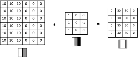
ViTs garnered a lot of hype because the team at Google Brain proved that they were viable alternatives to CNNs. CNNs, as their name suggests, are built using convolutional filters. In Figure 1 below, we have a 6x6 input matrix on the left, a 3x3 convolutional filter in the middle, and a 4x4 output tensor on the right. The output tensor’s values are calculated by multiplying each 3x3 section of the input matrix on the left with the 3x3 convolutional filter.
This particular convolutional filter, with positive 1 values in its left column, 0 values in its middle column, and negative 1 values in its right column, produces positive output values where vertical edges are found in the original matrix, i.e. in the middle of the example input matrix.
Figure 1: Convolutional filter for detecting vertical edges
The important thing to note from the above example is that convolutional filters, like this vertical edge detection filter, learn local features within an image. CNNs have many of these filters and each filter learns what values will extract the most meaningful information from the input image, but each filter only considers information in a localized window of the input image, e.g. a 3x3 crop of the image.
By stacking layers of these convolutional filters on top of one another, i.e. creating deep neural networks (DNNs), these local filters gradually gain greater attention over more abstract patterns that exist in larger sections of the image because they are consuming as inputs the filter outputs from a collection of adjacent local filters. We can see this progression of learned abstractions – from edges, to textures, to patterns, to object parts, to full objects – by inspecting the intermediate layers of DNNs at different depths as depicted below in Figure 2.
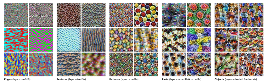
Figure 2: Progression of learned abstractions by visualizing features of a pre-trained DNN at increasingly deep layers. Original image available in this blog post by Google Research team.
Vision transformers are revolutionary because they employ global attention at each layer. Attention, as introduced in the paper “Attention is All You Need“, is a dense mapping of weights between different elements in a sequence. These weights represent the relative importance of each element in the sequence to all other elements in the sequence.
To more intuitively understand attention, take a look at the sentence below:
"I poured water from the bottle into the cup until it was full."
We might infer that the “it“ pronoun is referring to the “cup“ noun in this sentence because of the adjective “full“; however, by changing the word “full” to “empty”, the reference object for “it” changes from “cup” to “bottle“. We change this inference without much thought because of the innate knowledge we have about how the verb “pour” works, i.e., the act of pouring implies that the bottle is losing water and the cup is gaining water. This example demonstrates the relative importance of the word “full” to the context of the word “it” in this sentence.
Notice that in this example does not consider groups of three words at a time, but instead considered the entire sentence at the same time. Conceptually, this is what it means to have global attention and it can be very useful in comparison to local attention in inferring context within a problem space.
There’s just one significant problem with the concept of global attention employed by transformers: it’s a dense mapping and dense mappings scale quadratically.
In the above sentence, there are 13 words, i.e. N=13 elements in the sequence. To achieve global attention on this sequence, we need W=N*(N-1) or W=13*12=156 weights to represent the relative importance of each element to each other element (excluding ground truth class labels and patch delineators).
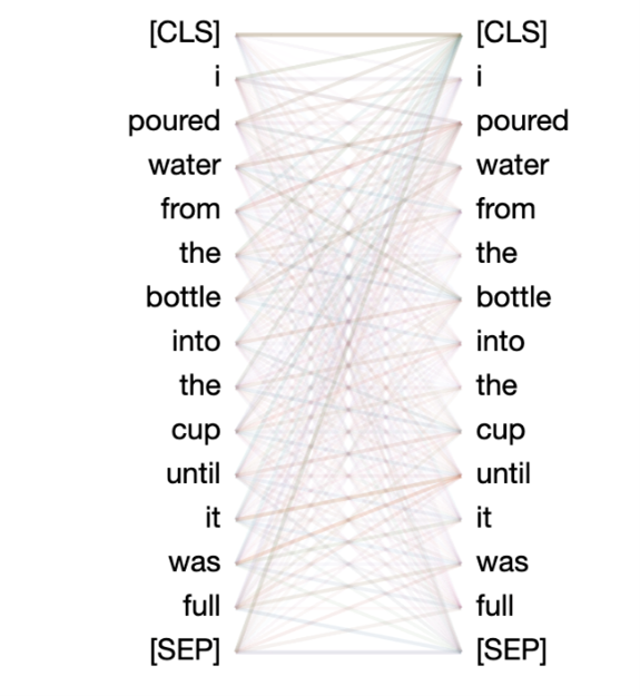
Figure 3: Visualization of an attention map.
This operation is expensive, but feasible for this two-dimensional data. Unfortunately, global attention becomes untenable when we try to adapt to higher dimensional data like RGB images used in computer vision applications, i.e. when N=224x224=50,176 pixels in an image and we need W=50176*(50175)=2,517,580,800 weights for global attention.
To solve this problem, ViTs preprocess the three-dimensional image data into a two-dimensional representation. They accomplish this by:
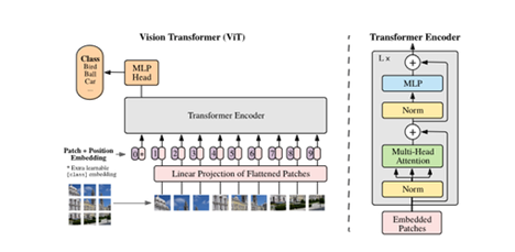
Figure 4: Depiction of image preprocessing required for Vision Transformers (ViT). Original image pulled from this paper.
To put it more simply, in traditional natural language transformers, the input sequences of data are sentences composed of words. Analogously in vision transformers, each image is a “sentence” and each patch embedding is a “word”.
At face value, these concepts do not seem to be so revolutionary. Dense or fully-connected layers were implemented as a part of Multilayer Perceptrons (MLP), the earliest proof-of-concept of neural networks. Similarly, the preprocessing needed for image vectorization is, fundamentally, just a form of mathematical embedding learned by a neural network.
To understand this why it's so hard to run ViT on most AI accelerators, we need to understand:
In Figure 4, we looked at an image focusing on the pre-processing needed to adapt three-dimensional image data to work with a transformer architecture. Below, in Figure 5, we zoom out to see what happens after the image data is preprocessed:
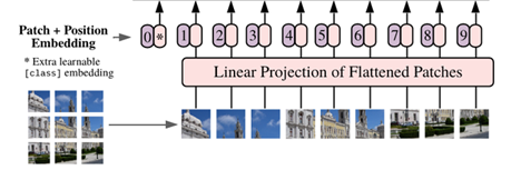
Figure 5: Entire Vision Transformer (ViT) architecture. Original image pulled from this paper.
Specifically, we want to look at the Transformer Encoder block on the right side of the image above. These encoder blocks are stacked L times for different sizes of ViT models, just like how ResNet-18 and ResNet-50 models are the same architecture with different numbers of stacked residual blocks.
The key differences to note between the ViT Encoder block and most CNN blocks is that it has normalization (represented as Norm layers in Figure 5) and softmax layers (the activation function used for the MLP layer in Figure 5) in the middle of the network. In almost all CNN architectures, normalization is performed once at the beginning of inference and Softmax is performed once at the end of the network.
Normalization and softmax layers are simple enough mathematical operations that do operate on large tensors in the context of DNNs. The challenge these pose to many AI SoCs targeting the edge is that they cannot be accelerated by linear algebra accelerators and in heterogeneous compute platforms need to be processed by a DSP, GPU, or CPU.
Heterogeneous compute nodes are computing devices with different architectures optimized for specific tasks, e.g. an AI SoC might include a CPU, a DSP, and an NPU like the design on the left in Figure 6 below:
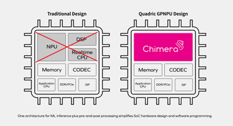
Figure 6: A heterogeneous AI SoC design with a dedicated NPU, DSP and CPU (left) compared with a homogeneous SoC design with a single, Chimera general-purpose NPU (GPNPU) processor core (right). Original image pulled from Quadric website.
Heterogeneous computing, as a design principle for AI, requires that programs be segmented into their component tasks and each task must target its most optimal compute node for runtime. If programmed or compiled incorrectly to target an inefficient compute node, e.g. the CPU instead of the AI accelerator, the runtime performance of the program can suffer greatly.
Heterogeneous computing platforms, and the NPU cores used within them, have been optimized for performance on most CNNs. Since most CNNs do not have any softmax or normalization operators in the middle of the network, most NPUs have been designed to optimize for only the convolutional compute which is just basic linear algebra.
NPUs have optimized for these multiply-accumulate (MAC) operations that constitute linear algebra math with great success and heterogeneous computing platforms that use these NPUs have excelled at running CNNs because there’s very infrequent, if any, data movement between compute nodes during inference. The entire inference program can be easily pipelined into three stages:
Heterogeneous computing platforms can hide most of the expensive memory-movement operations in these types of programs by pipelining the compute. Latency, or the time it takes to run the first inference, may be long, but throughput, the time it takes to run inference on average, is only limited by the slowest stage in this pipeline.
This runtime strategy, when applied to ViT architectures, creates a pipeline that requires frequent data movement between the different compute nodes:
This frequent movement of intermediate tensors between different compute nodes results in complex scheduling algorithms and significant overhead. This overhead of moving data between compute nodes substantially reduces the runtime efficiency of a model and burns excessive power. In AI SoC targeting power-sensitive edge applications, those extra memory-movement operations may render the system unviable.
Optimizing AI SoCs for performance on CNNs has enabled a lack of curiosity surrounding how to accelerate inference broadly. Heterogeneous computing platforms are using existing hardware IP and optimizing it for performance on AI tasks using complex software tricks. The only new hardware block that has been invented to address AI applications is the NPU and it was assumed that the only operations it would need to accelerate were MAC operations that make up the convolutional and dense layers in the middle of CNNs. The pervasiveness of this mindset can be seen by some NPU developers reporting model complexity in number of MAC operations. If MAC counts alone were indicative of a model’s complexity, ViTs would not be so challenging to run on AI SoCs that are optimized with these assumptions.
The SoC for AI applications that most easily adapts to new model architectures, like vision transformers, will win in the market long-term because:
© Copyright 2025 Quadric All Rights Reserved Privacy Policy